728x90
반응형
검증 목표
resnet50 모델을 사용하여 이미지 전체 데이터에 관해서 임베딩을 하여 유사한 거리에 있는 이미지를 추천한다.
사전준비
이미지 분류가 되어있는 폴더 안에 이미지가 N장 준비되어 있다.
이 파일들을 가지고 데이터셋을 생성하고 유사도를 검증해 볼 생각이다.

데이터셋 준비
from mpl_toolkits.mplot3d import Axes3D
from sklearn.preprocessing import StandardScaler
import matplotlib.pyplot as plt
import matplotlib.image as mpimg
import numpy as np
import pandas as pd
import os
import sklearn
# 데이터가 많으므로 테스트에서는 1000건만 처리하도록 한다.
NUM_ROWS = 1000
DATASET_PATH = "D:\\dataset\\sample"
print(os.listdir(DATASET_PATH))# ['bag', 'coat', 'jacket', 'shirt', 'skirt']categories = []
filenames = []
images = []
df = pd.DataFrame(columns=['category', 'filename', 'image'])
for folder in os.listdir(DATASET_PATH):
for file in os.listdir(os.path.join(DATASET_PATH, folder)):
categories.append(folder)
filenames.append(file)
images.append(os.path.join(DATASET_PATH, folder, file))
df['category'] = categories
df['filename'] = filenames
df['image'] = images
df = df.iloc[np.random.permutation(df.index)].reset_index(drop=True)
df = df[:NUM_ROWS]
df.head(10)| category | filename | image | |
| 0 | coat | sample1.jpg | D:\dataset\sample\sample1.jpg |
| 1 | shirt | sample2.jpg | D:\dataset\sample\sample2.jpg |
| 2 | shirt | sample3.jpg | D:\dataset\sample\sample3.jpg |
이미지 시각화
import cv2
import matplotlib.pyplot as plt
import numpy as np
# 딕셔너리 데이터를 인자값을 받아서 이미지를 출력한다.
def plot_figures(figures, nrows = 1, ncols=1,figsize=(5, 3)):
fig, axeslist = plt.subplots(ncols=ncols, nrows=nrows, figsize=figsize)
for ind,title in enumerate(figures):
axeslist.ravel()[ind].imshow(cv2.cvtColor(figures[title], cv2.COLOR_BGR2RGB))
axeslist.ravel()[ind].set_title(title)
axeslist.ravel()[ind].set_axis_off()
plt.tight_layout()# 이미지 경로를 읽어서 numpy로 변환한다.
# 기본 0.1 비율로 리사이즈를 처리한다.
def load_image(img_path, resized_fac = 0.1):
img = cv2.imread(img_path)
w, h, _ = img.shape
resized = cv2.resize(img, (int(h*resized_fac), int(w*resized_fac)), interpolation = cv2.INTER_AREA)
return resizedfigures = {'sample'+str(i) : load_image(row.image) for i, row in df.sample(6).iterrows()}
figures.keys()
plot_figures(figures, 2, 3)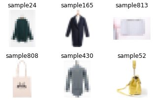
# 막대 그래프로 타입별로 갯수 출력
plt.figure(figsize=(6, 3))
df.category.value_counts().sort_values().plot(kind='barh')
추천 모델 (resnet50) 사용
import tensorflow as tf
import keras
from keras import Model
from keras.applications.resnet50 import ResNet50
from keras.preprocessing import image
from keras.applications.resnet50 import preprocess_input, decode_predictions
from keras.layers import GlobalMaxPooling2D
tf.__version__
# 입력 이미지
img_width, img_height, img_channel = 224, 224, 3
# 훈련된 모델 사용
base_model = ResNet50(weights='imagenet', include_top=False, input_shape = (img_width, img_height, img_channel))
base_model.trainable = False
model = keras.Sequential([
base_model,
GlobalMaxPooling2D()
])
model.summary()Model: "sequential_4"
_________________________________________________________________
Layer (type) Output Shape Param #
=================================================================
resnet50 (Model) (None, 7, 7, 2048) 23587712
_________________________________________________________________
global_max_pooling2d_4 (Glob (None, 2048) 0
=================================================================
Total params: 23,587,712
Trainable params: 0
Non-trainable params: 23,587,712
_________________________________________________________________전체 데이터 임베딩
def get_embedding(model, img_path):
    # Pillow 이미지 로드
    img = image.load_img(img_path, target_size=(img_width, img_height))
    # numpy 데이터로 변환 (224, 224, 3)
    x = image.img_to_array(img)
    # 차원을 추가해준다. (1, 224, 224, 3)
    x = np.expand_dims(x, axis=0)
    x = preprocess_input(x)
    # 1차원의 배열로 재배열해준다. [[5.232, 2.12, ...]] -> [5.232, 2.12, ...]
    return model.predict(x).reshape(-1)
# 첫 행 이미지 임베딩을 출력
emb = get_embedding(model, df.iloc[0].image)
emb.shape# (2048,)# 첫 행 이미지 시각화
img_array = load_image(df.iloc[0].image)
plt.figure(figsize = (2,2))
plt.imshow(cv2.cvtColor(img_array, cv2.COLOR_BGR2RGB))
print(img_array.shape)
print(emb)# (42, 30, 3)
# [2.853276 8.025141 1.2043287 ... 0.17113084 0.45344853 8.057759 ]
%%time

# 전체 데이터 임베딩
df_sample = df
map_embeddings = df_sample['image'].apply(lambda img: get_embedding(model, img))
df_embs = map_embeddings.apply(pd.Series)

print(df_embs.shape)
df_embs.head()
(1000, 2048)
Wall time: 49.5 s
| 0 | 1 | 2 | 3 | 4 | 5 | 6 | ... | 2041 | 2042 | 2043 | 2044 | 2045 | 2046 | 2047 | |
| 0 | 2.853276 | 8.025141 | 1.204329 | 3.509995 | 0.000000 | 0.017224 | 4.020164 | ... | 4.926272 | 9.721059 | 0.627201 | 2.847900 | 0.171131 | 0.453449 | 8.057759 |
| 1 | 11.037901 | 9.610494 | 3.251422 | 1.841570 | 6.155855 | 0.300533 | 0.000000 | ... | 3.231823 | 2.324785 | 2.415266 | 2.873397 | 3.033442 | 4.273942 | 9.356295 |
| 2 | 6.249569 | 11.492823 | 1.310759 | 0.000000 | 2.659937 | 1.060947 | 6.596041 | ... | 0.120667 | 0.000000 | 0.000000 | 1.862307 | 3.581021 | 3.856775 | 14.282220 |
| 3 | 4.452656 | 15.125280 | 3.368266 | 3.561770 | 0.000000 | 2.316134 | 3.634057 | ... | 0.000000 | 0.000000 | 0.623373 | 3.606657 | 0.000000 | 5.177092 | 9.513126 |
| 4 | 4.157537 | 9.734614 | 0.429734 | 1.033624 | 2.846768 | 0.000000 | 3.768886 | ... | 0.000000 | 2.047260 | 0.438755 | 4.212311 | 0.000000 | 1.660256 | 12.978857 |
5 rows × 2048 columns
유사도 계산
from sklearn.metrics.pairwise import pairwise_distances

# cosine 거리 계산
pairwise_distances(df_embs, metric='cosine')

# 정규화
cosine_sim = 1 - pairwise_distances(df_embs, metric='cosine')
cosine_sim[:4, :4]
array([[1. , 0.6729132 , 0.7783639 , 0.7777964 ],
[0.6729132 , 1. , 0.68061113, 0.6479302 ],
[0.7783639 , 0.68061113, 0.99999917, 0.6702682 ],
[0.7777964 , 0.6479302 , 0.6702682 , 0.9999989 ]], dtype=float32)유사한 이미지
가까운 거리에 있는 유사한 이미지를 출력한다.
indices = pd.Series(range(len(df)), index=df.index)

def get_recommender(idx, df, top_n = 5):
    sim_idx = indices[idx]
    sim_scores = list(enumerate(cosine_sim[sim_idx]))
    sim_scores = sorted(sim_scores, key=lambda x: x[1], reverse=True)
    sim_scores = sim_scores[1:top_n+1]
    idx_rec    = [i[0] for i in sim_scores]
    idx_sim    = [i[1] for i in sim_scores]

    return indices.iloc[idx_rec].index, idx_sim
# 유사한 데이터 출력해보기
idx_ref = 1
idx_rec, idx_sim = get_recommender(idx_ref, df, top_n = 6)
plt.figure(figsize = (2,2))
plt.imshow(cv2.cvtColor(load_image(df.iloc[idx_ref].image), cv2.COLOR_BGR2RGB))
figures = {'img-'+str(i): load_image(row.image) for i, row in df.loc[idx_rec].iterrows()}
plot_figures(figures, 2, 3)

임베딩 시각화
from sklearn.manifold import TSNE
import time
import seaborn as sns
time_start = time.time()
tsne = TSNE(n_components=2, verbose=0, perplexity=40, n_iter=300)
tsne_results = tsne.fit_transform(df_embs)
print('t-SNE done! Time elapsed: {} seconds'.format(time.time()-time_start))df['number'] = tsne_results[:,0]
df['distance'] = tsne_results[:,1]
plt.figure(figsize=(10,6))
sns.scatterplot(x="number", y="distance", hue="category", data=df, legend="full", alpha=0.8)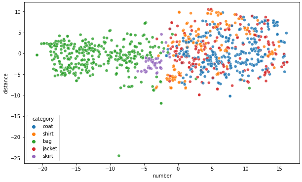
728x90
반응형
'AI 인공지능 > AI Vision' 카테고리의 다른 글
| YOLOv7에 대해 알아보자 (0) | 2022.11.22 |
|---|---|
| YOLOv7를 활용한 Object Detection (0) | 2022.11.21 |
| 패션 의류 분류 (Fashion Classification) (0) | 2021.09.15 |
| Fashion MNIST (0) | 2021.09.12 |
| Object Detection 개념 (0) | 2021.09.12 |


